1. Introduction
Machine learning has become one of the most impactful fields in modern technology — influencing recommendation systems, medical diagnosis, autonomous vehicles, and generative AI. At its core, machine learning enables systems to recognize patterns in data and use those patterns to make decisions or produce meaningful outputs.
Depending on how learning is structured, machine learning is broadly categorized into supervised, unsupervised, reinforcement learning, and self-supervised learning:
- Supervised learning trains on labelled pairs (x, y) to predict outputs for new inputs — used in classification and regression.
- Unsupervised learning uncovers hidden structure in unlabelled data — clustering and dimensionality reduction.
- Reinforcement learning trains through reward-and-punishment feedback loops.
- Self-supervised learning generates supervision signals from the data itself — e.g., predicting the next token in text.
Within these paradigms, two fundamental model categories emerge: predictive (discriminative) models and generative models. Predictive models focus on mapping inputs to outputs efficiently. Generative models aim to understand the underlying data distribution so they can synthesize new samples. This distinction — seemingly simple — leads to profound differences in architecture, training objectives, and capabilities.
2. Predictive Models
Predictive models have a clear objective: given an input $x$, produce the most accurate output $y$ possible. They learn the conditional probability $P(Y \mid X)$ — the likelihood of a label given an observation — without needing to model how the data itself was generated.
This focused approach makes them highly efficient. Training optimizes a loss function that penalizes deviations from true labels:
- Mean Squared Error (MSE) for regression tasks.
- Cross-Entropy Loss for classification — maximizing the probability of correct class predictions.
A key characteristic is the decision boundary. Logistic regression finds a linear boundary; neural networks learn complex non-linear surfaces. Because they do not model the full distribution $P(X)$, predictive models train faster, require less compute, and generally need less data — but they cannot generate new data samples.
3. Generative Models
Generative models take a fundamentally different approach: instead of only predicting labels, they aim to understand how data is generated. This means learning the joint distribution $P(X, Y)$, decomposed as $P(X \mid Y)\,P(Y)$, so that new samples can be drawn from it.
A central concept is the latent space — a lower-dimensional representation that encodes essential properties of the data. Sampling from this latent space produces new, realistic data points.
Training generative models is significantly more complex. Common approaches include:
- Maximizing log-likelihood of observed data under the model.
- Adversarial training (GANs) — a generator and discriminator in competition.
- Variational inference (VAEs) — optimizing a lower bound on log-likelihood.
- Score matching / denoising (Diffusion models).
4. Types of Models
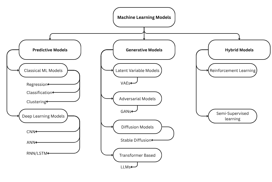
Figure 1 — Machine Learning Model Taxonomy
4.1 Predictive Model Types
Classical methods:
- Linear / Logistic Regression — fast baselines for regression and binary classification.
- Support Vector Machines (SVM) — effective in high-dimensional spaces with clear margins.
- Decision Trees / Random Forests / Gradient Boosting — strong on tabular data; GBT methods (XGBoost, LightGBM) dominate competitive ML.
- K-Nearest Neighbours (KNN) — instance-based, non-parametric, excellent for local structure.
Deep learning methods:
- CNNs — hierarchical feature extraction for images and video.
- RNNs / LSTMs — sequential modelling for time-series and text.
- Transformers — now dominant across NLP, vision, and multimodal tasks via attention.
4.2 Generative Model Types
- Variational Autoencoders (VAEs) — encoder compresses input to a probabilistic latent code; decoder reconstructs. Enables smooth, interpolable latent spaces.
- Generative Adversarial Networks (GANs) — generator vs. discriminator minimax game. Produces extremely sharp outputs but is notoriously unstable (mode collapse).
- Diffusion Models — add noise iteratively, then learn to reverse. Currently state-of-the-art for image synthesis (Stable Diffusion, DALL·E 3, Imagen).
- Autoregressive Transformers (LLMs) — generate data one token at a time conditioned on context. Powers GPT, LLaMA, Gemini.
- Normalizing Flows — exact likelihood estimation via invertible transformations.
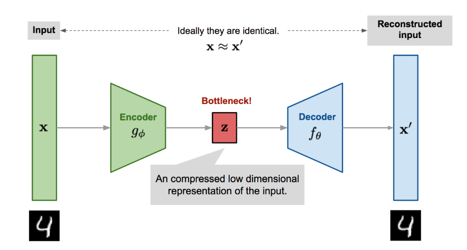
Figure 2 — Variational Autoencoder (VAE) Architecture
5. Comparative Analysis
| Aspect | Predictive Models | Generative Models |
|---|---|---|
| Probability Modeled | $P(Y|X)$ — Conditional | $P(X, Y)$ — Joint |
| Primary Goal | Predict output from input | Learn & synthesize data distribution |
| Data Requirement | Requires labelled data | Can use unlabelled data |
| Can Classify | Yes — primary purpose | Yes — via Bayes' rule |
| Can Generate Data | No | Yes — core capability |
| Training Complexity | Lower — faster convergence | Higher — harder to stabilize |
| Data Dependence | Heavy reliance on labelled history | Less dependent; learns distribution |
| Interpretability | Generally more interpretable | Often "black box" |
| Examples | SVM, Random Forest, BERT, CNN | VAE, GAN, Diffusion, GPT |
Evaluation Metrics
- Predictive models: Accuracy, Precision, Recall, F1-Score, AUC-ROC, MSE/RMSE.
- Generative models: Fréchet Inception Distance (FID), Inception Score (IS), Perplexity, Reconstruction Loss (MSE / BCE).
6. Applications
Predictive Model Applications
- Medical diagnosis — disease prediction from patient records and imaging.
- Fraud detection — anomaly flagging in financial transactions.
- Recommendation systems — content and product personalization at scale.
- Demand forecasting — inventory planning and resource allocation.
- Credit risk assessment — probability of loan default estimation.
- NLP classification — spam detection, sentiment analysis, intent recognition.
Generative Model Applications
- Image / video synthesis — photorealistic media generation (Midjourney, DALL·E, Sora).
- Text generation — conversational AI, code generation, document writing (GPT-4, Claude).
- Data augmentation — synthetic training data to address class imbalance.
- Drug discovery — molecular structure generation with targeted properties.
- Image restoration — inpainting, super-resolution, style transfer.
- Anomaly detection — flagging deviations from the learned normal distribution.
7. Experiments on MNIST
7.1 Dataset
MNIST handwritten digits (0–9): 28×28 grayscale images, loaded from hojjatk/mnist-dataset via KaggleHub (IDX binary format). 60,000 training / 10,000 test samples.
7.2 Predictive Experiment — Logistic Regression & KNN
End-to-end supervised workflow with preprocessing (flatten, normalize), hyperparameter tuning, metric logging, and confusion matrix analysis.
Softmax probability for class $c$:
$$p_\theta(y=c \mid x_i) = \frac{\exp(w_c^\top x_i + b_c)}{\sum_k \exp(w_k^\top x_i + b_k)}$$SGD parameter update:
$$\theta_{t+1} = \theta_t - \eta \,\nabla_\theta \mathcal{L}_{\text{log-loss}}(\theta_t)$$Multiclass cross-entropy loss:
$$\mathcal{L}_{\text{log-loss}} = -\frac{1}{N}\sum_{i=1}^{N}\sum_{c} y_{ic}\,\log\, p_\theta(y=c \mid x_i)$$7.3 Generative Experiment — VAE
End-to-end VAE workflow: encoder learns approximate posterior, reparameterisation trick enables backprop through stochastic latent, decoder reconstructs/generates digits.
Encoder posterior & decoder:
$$q_\phi(z \mid x) = \mathcal{N}\!\left(\mu_\phi(x),\,\operatorname{diag}(\sigma_\phi^2(x))\right), \quad p_\theta(x \mid z)$$Reparameterisation trick:
$$z = \mu_\phi(x) + \sigma_\phi(x) \odot \varepsilon, \quad \varepsilon \sim \mathcal{N}(0,\,I)$$VAE ELBO objective (negative ELBO to minimize):
$$\mathcal{L}_{\text{VAE}} = \mathcal{L}_{\text{recon}}(x, \hat{x}) + D_{\mathrm{KL}}\!\left(q_\phi(z \mid x) \,\|\, p(z)\right)$$Reconstruction uses binary cross-entropy during training. For reporting, quality is measured as MSE:
$$\text{MSE} = \frac{1}{N}\sum_{i=1}^{N}\lVert x_i - \hat{x}_i \rVert_2^2$$7.4 Results
| Model | Accuracy | Precision | Recall | F1 | Recon. Loss |
|---|---|---|---|---|---|
| Logistic Regression (SGD) | 90.69% | 0.9065 | 0.9069 | 0.9065 | N/A |
| KNN (K = 3) | 97.14% | — | — | 0.9714 | N/A |
| KNN (K = 5) | 96.96% | — | — | 0.9696 | N/A |
| Variational Autoencoder | N/A | N/A | N/A | N/A | 0.014226 |
7.5 Observations
- Logistic Regression provides a clean 90.69% baseline with no tuning — solid for a linear model on 784-dimensional input.
- KNN at K=3 achieves 97.14%, showing that local geometry is highly informative for digit recognition.
- The VAE reconstruction loss of 0.0142 demonstrates high-quality digit reconstruction — visually indistinguishable from originals on most samples.
- The fundamental trade-off is clear: predictive models optimize for discrimination; generative models optimize for synthesis. Both are useful; the choice depends entirely on the downstream task.
8. Conclusion
Predictive and generative models represent two complementary paradigms in machine learning. Predictive models excel at efficiently mapping inputs to accurate outputs — they are faster to train, easier to interpret, and highly performant on classification and regression tasks across structured domains.
Generative models provide the ability to understand, compress, and recreate data distributions — enabling powerful applications in content synthesis, data augmentation, anomaly detection, and scientific discovery. They are less dependent on labelled data but significantly more complex to train and evaluate.
In modern systems, both paradigms are often combined: a generative model augments the training set, and a predictive model achieves higher accuracy as a result. Understanding the strengths and trade-offs of each is fundamental knowledge for any machine learning practitioner.
9. References
- [1] J. Ho, A. Jain, P. Abbeel — "Denoising Diffusion Probabilistic Models," arXiv:2006.11239, 2020. ↗
- [2] I. Goodfellow et al. — "Generative Adversarial Networks," arXiv:1406.2661, 2014. ↗
- [3] D. P. Kingma, M. Welling — "Auto-Encoding Variational Bayes," arXiv:1312.6114, 2014. ↗
- [4] A. Y. Ng, M. I. Jordan — "On Discriminative vs. Generative Classifiers," NeurIPS, 2001. ↗
- [5] A. Vaswani et al. — "Attention Is All You Need," arXiv:1706.03762, 2017. ↗
- [6] C. Zheng et al. — "Revisiting Discriminative vs. Generative Classifiers," arXiv:2302.02334, 2023. ↗